Hashing, Hash Data Structure and Hash Table

Hashing is the process of mapping large amount of data item to a smaller table with the help of a hashing function. The essence of hashing is to facilitate the next level searching method when compared with the linear or binary search. The advantage of this searching method is its efficiency to hand vast amount of data items in a given collection (i.e. collection size).

Due to this hashing process, the result is a Hash data structure that can store or retrieve data items in an average time disregard to the collection size.

Hash Table is the result of storing the hash data structure in a smaller table which incorporates the hash function within itself. The Hash Function primarily is responsible to map between the original data item and the smaller table itself. Here the mapping takes place with the help of an output integer in a consistent range produced when a given data item (any data type) is provided for storage and this output integer range determines the location in the smaller table for the data item. In terms of implementation, the hash table is constructed with the help of an array and the indices of this array are associated to the output integer range.

Hash Table Example :
Here, we construct a hash table for storing and retrieving data related to the citizens of a county and the social-security number of citizens are used as the indices of the array implementation (i.e. key). Let's assume that the table size is 12, therefore the hash function would be Value modulus of 12.

Hence, the Hash Function would equate to:
(sum of numeric values of the characters in the data item) %12
Note! % is the modulus operator

Let us consider the following social-security numbers and produce a hashcode:
120388113D => 1+2+0+3+8+8+1+1+3+13=40
Hence, (40)%12 => Hashcode=4

310181312E => 3+1+0+1+8+1+3+1+2+14=34
Hence, (34)%12 => Hashcode=10

041176438A => 0+4+1+1+7+6+4+3+8+10=44
Hence, (44)%12 => Hashcode=8

Therefore, the Hashtable content would be as follows:
-----------------------------------------------------
0:empty
1:empty
2:empty
3:empty
4:occupied Name:Drew Smith SSN:120388113D
5:empty
6:empty
7:empty
8:occupied Name:Andy Conn SSN:041176438A
9:empty
10:occupied Name:Igor Barton SSN:310181312E
11:empty
-----------------------------------------------------

Find shortest path using Dijkstra's Algorithm

The Dijkstra's algorithm entails the following procedure:
- The breath-first approach is used to traversal the network, however the difference here is instead of a queue data structure to store the traversed vertex this algorithm uses a priority queue. The priority queue helps to remove the items in order of values rather than in order of being added to the queue.
- Have an account of lowest total path weight (i.e. weightsum), from the start vertex to the target vertex
- Have an account of immediate predecessor in a given path for each vertex
- Have an account of the items in the priority queue

Exercise- Find the shortest path from Pori to Kuopio


1
----------------------------------------------------
Vertex - Weightsum - Predecessor
----------------------------------------------------
Helsinki - nul - null
Ivalo - null - null
Kouvola - null - null
Kuopio - 409 - Pori
Oulu - null - null
Pori - 0 - Pori
Tampere - 110 - Pori
Turku - 141 - Pori
----------------------------------------------------
Visited: Pori
Priority Queue: (Tampere,110), (Turku,141), (Kuopio,409)

2
----------------------------------------------------
Vertex - Weightsum - Predecessor
----------------------------------------------------
Helsinki - 287 - Tampere
Ivalo - null - null
Kouvola - null - null
Kuopio - 404 - Tampere
Oulu - null - null
Pori - 0 - Pori
Tampere - 110 - Pori
Turku - 141 - Pori
----------------------------------------------------
Visited: Pori,(Tampere,110)
Priority Queue: (Turku,141),(Helsinki,287),(Kuopio,404),(Kuopio,409)

3
----------------------------------------------------
Vertex - Weightsum - Predecessor
----------------------------------------------------
Helsinki - 287 - Tampere
Ivalo - null - null
Kouvola - null - null
Kuopio - 404 - Tampere
Oulu - null - null
Pori - 0 - Pori
Tampere - 110 - Pori
Turku - 141 - Pori
----------------------------------------------------
Visited: Pori,(Tampere,110),(Turku,141)
Priority Queue: (Helsinki,287),(Kuopio,404),(Kuopio,409)

4
----------------------------------------------------
Vertex - Weightsum - Predecessor
----------------------------------------------------
Helsinki - 287 - Tampere
Ivalo - null - null
Kouvola - 364 - Helsinki
Kuopio - 404 - Tampere
Oulu - null - null
Pori - 0 - Pori
Tampere - 110 - Pori
Turku - 141 - Pori
----------------------------------------------------
Visited: Pori,(Tampere,110),(Turku,141),(Helsinki,287)
Priority Queue: (Kouvola,364),(Kuopio,404),(Kuopio,409)

5
----------------------------------------------------
Vertex - Weightsum - Predecessor
----------------------------------------------------
Helsinki - 287 - Tampere
Ivalo - null - null
Kouvola - 364 - Helsinki
Kuopio - 404 - Tampere
Oulu - 898 - Kouvola
Pori - 0 - Pori
Tampere - 110 - Pori
Turku - 141 - Pori
----------------------------------------------------
Visited: Pori,(Tampere,110),(Turku,141),(Helsinki,287),(Kouvola,364)
Priority Queue: (Kuopio,404),(Kuopio,409),(Oulu,898)

6
----------------------------------------------------
Vertex - Weightsum - Predecessor
----------------------------------------------------
Helsinki - 287 - Tampere
Ivalo - null - null
Kouvola - 364 - Helsinki
Kuopio - 404 - Tampere
Oulu - 898 - Kouvola
Pori - 0 - Pori
Tampere - 110 - Pori
Turku - 141 - Pori
----------------------------------------------------
Visited: Pori,(Tampere,110),(Turku,141),(Helsinki,287),(Kouvola,364),(Kuopio,404)
Priority Queue: (Kuopio,409),(Oulu,898)

Therefore the shortest path from Pori to Kuopio is Pori,(Tampere,110),(Kuopio,404)

What is a Network in the context of Graph?

Network refers to a graph in which the edges are bound with weights. Here weights can be numbers assigned to a the edges. Hence, a graph of this nature is referred to as weighted graph or a network.

Graph Traversal Methods

There are two possible traversal methods for a graph:
i. Breadth-First Traversal
ii. Depth-First Traversal

i. Breadth-First Traversal: Traverse all the vertices starting from a given 'start vertex'. Hence, such a traversal follows the 'neighbour-first' principle by considering the following:
- No vertex is visited more than once
- Only those vertices that can be reached are visited

Importantly here, we make use of the Queue data structure. In effect, we house the vertices in the queue that are to be visited soon in the order which they are added to this queue i.e. first-in first-out.

Visiting a vertex involves returning the data item in the vertex and adding its neighbour vertices to the queue. However, we don't carryout any action under following conditions:
- if the neighbour is already present in the queue or if the neighbour has been already visited

As an example of the breadth-first traversal, we traverse the major cities of Finland with by the start vertex as 'Pori . Note! the neighbour(s) of a given vertex are added to the queue in alphabetical order.



1
Visited: Pori
Queue: Tampere, Turku

2
Visited: Pori, Tampere
Queue: Turku, Helsinki, Kuopio

3
Visited: Pori, Tampere, Turku
Queue: Helsinki, Kuopio

4
Visited: Pori, Tampere, Turku, Helsinki
Queue: Kuopio, Kouvola

5
Visited: Pori, Tampere, Turku, Helsinki, Kuopio
Queue: Kouvola

6
Visited: Pori, Tampere, Turku, Helsinki, Kuopio, Kouvola
Queue: Oulu

7
Visited: Pori, Tampere, Turku, Helsinki, Kuopio, Kouvola, Oulu
Queue: empty

Therefore, the route yielded by the Breadth-First traversal:
Pori, Tampere, Turku, Helsinki, Kuopio, Kouvola, Oulu


ii. Depth-First Traversal: Traverse all the vertices starting from a given 'start vertex'. Hence, such a traversal follows the 'neighbour-first' principle by considering the following:
- No vertex is visited more than once
- Only those vertices that can be reached are visited

Importantly here, we make use of the Stack data structure. In effect, we stack the vertices so that vertices to be visited soon are in order in which they are popped from the stack i.e. last-in, first-out.

Visiting a vertex involves returning the data item in the vertex and adding its neighbour vertices to the stack. However, we don't carryout any action if the following occurs:
- neighbour is already present in the stack or if the neighbour has already been visited


As an example of the depth-first traversal, we traverse the major cities of Finland with by the start vertex as 'Pori'. Note! the neighbour(s) of a given vertex are pushed to the stack in alphabetical order.

1
Visited: Pori
Stack:
-------
Turku
-------
Tampere
-------

2
Visited: Pori, Turku
Stack:
-------
Helsinki
-------
Tampere
-------

3
Visited: Pori, Turku, Helsinki
Stack:
-------
Kuopio
-------
Kouvola
-------
Tampere
-------

4
Visited: Pori, Turku, Helsinki, Kuopio
Stack:
-------
Kouvola
-------
Tampere
-------

5
Visited: Pori, Turku, Helsinki, Kuopio, Kouvola
Stack:
-------
Oulu
-------
Tampere
-------

6
Visited: Pori, Turku, Helsinki, Kuopio, Kouvola, Oulu
Stack:
-------
Tampere
-------

7
Visited: Pori, Turku, Helsinki, Kuopio, Kouvola, Oulu, Tampere
Stack:
-------
Empty
-------

Therefore, the route yielded by the Depth-First traversal:
Pori, Turku, Helsinki, Kuopio, Kouvola, Oulu, Tampere

Types of Graphs

There two types of graphs:
i. Undirected Graphs
ii. Directed Graphs

Undirected Graph: A graph that entail edges with ordered pair of vertices, however it does not have direction define. Example of such a graph is the 'Family tree of the Greek gods'

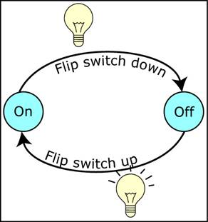
Directed Graph: A graph that entail edges with ordered pair of vertices and has direction indicated with an arrow. Example of such a graph is the 'A finite-state machine of a light switch'

What is a Graph data structure?

Graph is an Abstract Data Type (ADT) which is of a non-linear structure entailing sets of nodes and connectors. Here, the connectors helps to establish relationship between nodes. However, from the graph ADT literature point-of-view the nodes are referred to as Vertices and connectors are referred to as Edges.
Mathematically, a graph G entails vertices V, which are connected by edges E. Hence, a graph is defined as an ordered pair G=(V,E), where V is a finite set and E is a set consisting of two element subsets of V.

What is Bucket Sort?

Bucket Sort (alternatively know as bin sort) is an algorithm that sorts numbers and comes under the category of distribution sort.
This sorting algorithm doesn't compare the numbers but distributes them, it works as follows:
1. Partition a given array into a number of buckets
2. One-by-one the numbers in the array are placed in the designated bucket
3. Now, only sort the bucket that bare numbers by recursively applying this Bucket Sorting algorithm
4. Now, visiting the buckets in order, the numbers should be sorted